F1 Score: Precision-Recall Balance - January 2026

Published January 13, 202618 min read

Everyone checks data accuracy first. It's intuitive, easy to explain, and usually good enough when classes are balanced. But when positives make up 2% of your data, a model that predicts negative every time scores 98% accuracy while learning nothing useful. F1 score cuts through that by focusing only on how well you identify and classify the minority class. We'll cover the math, the trade-offs, and the practical steps for tuning and monitoring F1 in systems where imbalance is the norm.

TLDR:

F1 score balances precision and recall using harmonic mean, preventing models from gaming metrics
For imbalanced data, F1 ignores true negatives and focuses on minority class performance
Optimal classification thresholds rarely sit at 0.5; grid search across thresholds maximizes F1
Macro, micro, and weighted F1 variants handle multiclass problems with different class priorities
Openlayer automates F1 testing in CI/CD and monitors production drift with real-time alerts

Understanding F1 score and the confusion matrix

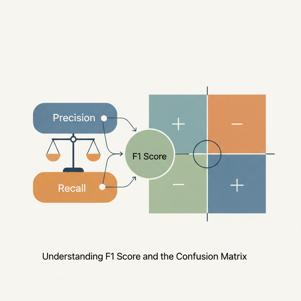
The F1 score is the harmonic mean of precision and recall. It condenses two competing metrics into a single value that penalizes extreme imbalances between them. The foundation lies in the confusion matrix: true positives (TP), false positives (FP), true negatives (TN), and false negatives (FN). Precision measures how many predicted positives were actually correct (TP / (TP + FP)). Recall measures how many actual positives you successfully identified (TP / (TP + FN)). The f1 score formula combines these: F1 = 2 × (Precision × Recall) / (Precision + Recall). The harmonic mean requires both metrics to be reasonably high for F1 to be high. A classifier with 90% precision but 10% recall yields an F1 of only 0.18, exposing the weakness that accuracy alone would mask.

This matters when class distributions are skewed or when false positives and false negatives carry different costs. In fraud detection, missing actual fraud (low recall) hurts even if you rarely flag legitimate transactions (high precision). F1 score surfaces that trade-off immediately.

Calculating the F1 score

So how do you calculate this score?

First, start with the precision-recall approach.
Next, given a confusion matrix, calculate precision first: divide true positives by all predicted positives (TP + FP).
Then, calculate recall: divide true positives by all actual positives (TP + FN).
Finally, apply the F1 formula: 2 × (Precision × Recall) / (Precision + Recall).

Here's a concrete example. Your binary classifier produces 85 true positives, 15 false positives, and 20 false negatives. Precision equals 85 / (85 + 15) = 0.85. Recall equals 85 / (85 + 20) ≈ 0.81. F1 becomes 2 × (0.85 × 0.81) / (0.85 + 0.81) ≈ 0.83. But, you can also derive F1 directly from confusion matrix counts. The f1 score formula in terms of true positives is: F1 = 2TP / (2TP + FP + FN). Using the same numbers: 2(85) / (2(85) + 15 + 20) = 170 / 205 ≈ 0.83.

The direct formula is faster when batch-processing results or integrating scoring into automated pipelines.

Why F1 score uses harmonic mean instead of arithmetic mean

As we mentioned previously, F1 is a harmonic mean. But what is that? The arithmetic mean of precision and recall would treat both metrics equally. A model with 100% precision and 0% recall would score 50%, suggesting moderate performance when the model predicts nothing useful. The harmonic mean, on the other hand, penalizes imbalances by weighting lower values more heavily, making it one of the key ML evaluation metrics. When one metric approaches zero, the harmonic mean collapses toward zero regardless of the other metric's strength.

Consider precision of 1.0 and recall of 0.1. The arithmetic mean yields 0.55. The harmonic mean produces 0.18, exposing a model that achieves high precision by barely identifying any positives. This property prevents gaming the evaluation. You cannot achieve a strong F1 score without reasonable performance in both precision and recall.

F1 score vs accuracy for model evaluation

Obviously, you have a choice when evaluating the efficacy of your model. You can either opt for F1 or use an accuracy measurement. How do these two approaches differ?

Accuracy measures the fraction of all predictions that were correct: (TP + TN) / (TP + TN + FP + FN). It treats every prediction equally, which works when classes are balanced and errors cost roughly the same. The problem surfaces with class imbalance. If 95% of transactions are legitimate, a classifier that always predicts "not fraud" achieves 95% accuracy while catching zero fraud cases. Accuracy rewards passivity when the majority class dominates.
F1 score ignores true negatives entirely. It focuses on how well you identify and correctly label the minority class. In the fraud example, precision and recall would both be undefined or zero, yielding an F1 of 0 and exposing the model's failure immediately.

The bottom line? Use accuracy when classes are balanced and all error types carry similar costs in your model evaluation in machine learning. Use F1 score when one class is rare, when false negatives are costly, or when you care about positive-class performance. For imbalanced datasets, F1 provides a more honest signal of whether your model solves the actual problem.

Digging into F1

Before you commit to F1, though, it's important to understand how to interpret score values and ranges as well as some specific cases you should consider.

Interpreting F1 score values and ranges

F1 scores range from 0.0 to 1.0, where 1.0 represents perfect precision and recall. A score of 0.0 indicates the model failed to correctly identify any true positives.

What counts as a good F1 score depends on your domain. Medical diagnosis systems targeting rare diseases might require F1 above 0.90 to be clinically useful. Spam filters often operate effectively between 0.75 and 0.85. Exploratory research models may start at 0.50 and improve through iteration.

Context matters more than absolute thresholds, though. An F1 of 0.70 represents strong performance in noisy domains with ambiguous ground truth but signals failure in high-stakes applications like financial fraud detection. As you implement F1, you should compare your score against baseline models, random classifiers, and domain-specific requirements instead of universal benchmarks to better optimize your F1 scoring.

Consideration #1: imbalanced datasets

Class imbalance exposes a weakness in most evaluation metrics: they reward models that exploit the majority class. When negatives outnumber positives 100:1, predicting the majority achieves high accuracy while learning nothing about the target. F1 score resists this by ignoring true negatives. Both precision and recall depend only on true positives, false positives, and false negatives. A model cannot inflate F1 by correctly classifying abundant negatives.

For imbalanced datasets, what is a good F1 score varies by how rare the positive class is. Detecting defects in manufacturing with 1% failure rates might achieve F1 of 0.60 after tuning. Credit default prediction with similar imbalance may target 0.75 or higher depending on the cost of missed defaults versus unnecessary credit denials. Weighted F1 score further extends this by averaging per-class F1 values scaled by class frequency, providing a single metric that accounts for all classes in multi-class imbalanced problems.

Consideration #2: optimizing classification thresholds

The goal should be to maximize your F1 score. But, most classifiers output probabilities instead of hard labels. The classification threshold determines which probability values map to positive predictions. The default threshold of 0.5 rarely maximizes F1 score. Moving the threshold changes the precision-recall trade-off. Lower thresholds increase recall by classifying more samples as positive but reduce precision by including more false positives. Higher thresholds do the opposite.

In addition, grid search evaluates F1 across threshold candidates from 0.0 to 1.0 in small increments during model validation, then selects the threshold yielding the highest score. For well-calibrated classifiers, research shows the optimal threshold approximates half the maximum F1 value, providing a useful starting point before fine-tuning.

Macro F1, micro F1, and weighted F1 score explained

Multiclass problems require aggregating per-class F1 scores. Three methods handle class contributions differently:

Macro F1
Micro F1
Weighted F1

Macro F1

Macro F1 calculates F1 for each class independently, then averages them. Each class receives equal weight regardless of sample count. A model that excels at majority classes but fails on rare ones will show a lower macro F1 than accuracy suggests. Use this when all classes matter equally, such as multi-disease diagnosis where rare conditions deserve the same attention as common ones.

Micro F1

Micro F1 pools all true positives, false positives, and false negatives across classes before computing a single precision, recall, and F1. This gives more weight to classes with more samples and behaves similarly to accuracy in balanced datasets. You should choose this when overall correctness matters more than per-class fairness.

Weighted F1

Weighted F1 calculates per-class F1 scores, then averages them proportionally to class frequency. This balances the class-agnostic view of macro with the volume sensitivity of micro. This approach works well for imbalanced datasets where you want to acknowledge class distributions without ignoring minority performance.

F1 score implementation with scikit-learn

Scikit-learn is an open-source machine learning library. According to their documentation, this library, "supports supervised and unsupervised learning. It also provides various tools for model fitting, data preprocessing, model selection, model evaluation, and many other utilities."

from sklearn.metrics import f1_score, classification_report

y_true = [0, 1, 1, 0, 1, 1, 0, 0, 1, 0]
y_pred = [0, 1, 1, 0, 0, 1, 0, 1, 1, 0]

binary_f1 = f1_score(y_true, y_pred)


For multiclass problems, specify the averaging method:

y_true_multi = [0, 1, 2, 0, 1, 2, 0, 1, 2]
y_pred_multi = [0, 2, 2, 0, 1, 1, 0, 1, 2]

macro = f1_score(y_true_multi, y_pred_multi, average='macro')
micro = f1_score(y_true_multi, y_pred_multi, average='micro')
weighted = f1_score(y_true_multi, y_pred_multi, average='weighted')

The classification_report() function outputs precision, recall, and F1 for all classes in a single call.

F-Beta score and adjusting precision-recall trade-offs

F1 can be extended through the F-Beta score which allows you to focus on precision or recall by adjusting the weight of each metric.

In this way, the F-beta score generalizes the F score by adding a β parameter that weights precision against recall: F-beta = (1 + β²) × (Precision × Recall) / (β² × Precision + Recall). Consider the following scenarios:

F1 sets β to 1, which reduces to the standard F1 formula.
F2 score sets β to 2, weighting recall twice as heavily as precision. Medical screening for serious diseases, for example, focuses catching all potential cases even if some false positives require follow-up testing. Missing a true case carries higher cost than an unnecessary test.
F0.5 score sets β to 0.5, weighting precision twice as heavily as recall. Spam filtering tolerates missing some spam if it prevents legitimate emails from being blocked. False positives frustrate users more than occasional spam in the inbox.

Adjusting β shifts emphasis. β values below 1 favor precision. β values above 1 favor recall. You should choose β based on business impact during AI model testing, not statistical preference.

Limitations and criticisms of F1 score

Of course, no evaluation criteria is ever perfect and F1 definitely has its detractors. Below are a few limitations and criticisms of F1 score:

F1 score ignores true negatives entirely. This makes it unsuitable for domains where correctly identifying negatives matters. In malware detection, knowing a file is clean carries as much value as catching malicious code.
The harmonic mean equally weights precision and recall without justification. Many applications assign different costs to false positives versus false negatives, yet F1 offers no mechanism to encode these trade-offs beyond switching to F-beta.
The metric lacks symmetry. Swapping positive and negative class labels produces different F1 scores even though the underlying classifier performance remains identical.

Matthews Correlation Coefficient (MCC) tackles these limitations by including all four confusion matrix values and remaining symmetric under class label swaps. MCC ranges from -1 to +1, where 0 represents random performance and negative values indicate predictions worse than chance.

The bottom line is that F1 remains useful for imbalanced positive-class-focused tasks but should not be your only evaluation metric. Combine it with precision-recall curves, MCC, or error analysis in machine learning. Combine it with precision-recall curves, MCC, or domain-specific cost functions that reflect actual constraints.

Testing and monitoring F1 score in production systems

Let's face it, decisions made in development are not always the best for production systems. So you should keep in mind some recommendations around testing and monitoring your F1 score once the system is in production:

F1 score evaluation extends beyond model training into production, where data distributions shift and model behavior drifts over time.
Automated ML evaluation testing pipelines assess F1 on validation sets before each deployment. When F1 drops below acceptable thresholds, the system blocks promotion and alerts engineering teams to prevent regressions from reaching users.
Live monitoring tracks F1 on production traffic by comparing predictions against delayed ground truth labels. Fraud detection systems receive actual fraud determinations days or weeks after initial predictions, allowing monitoring systems to compute rolling F1 scores and detect degradation.
Segmented analysis reveals performance gaps hidden by aggregate metrics. A model maintaining 0.82 overall F1 might show 0.65 F1 on a specific customer segment or geographic region, exposing disparities when sliced by cohort, time window, or feature value.
Alerting rules trigger when F1 falls outside control bounds or when precision-recall balance shifts unexpectedly. Sudden recall drops signal that the model stopped identifying positives, while precision drops indicate contamination from false positives.

Openlayer handles this testing and monitoring across development and production. F1 thresholds defined during model development become runtime guardrails in production, creating a closed feedback loop that catches issues before they compound.

Final thoughts on F1 score as an evaluation metric

F1 score vs accuracy becomes critical when class distributions skew or when false negatives carry different costs than false positives. The harmonic mean structure keeps you honest by collapsing toward zero when either precision or recall fails. Combine F1 with threshold optimization, segmented analysis, and continuous monitoring to maintain model quality from development through production. Choose your averaging method and beta parameter based on business impact, not statistical convenience.

FAQ

How do I calculate F1 score from a confusion matrix?

Divide true positives by the sum of true positives and false positives to get precision, then divide true positives by the sum of true positives and false negatives to get recall. Apply the formula: F1 = 2 × (Precision × Recall) / (Precision + Recall), or use the direct formula F1 = 2TP / (2TP + FP + FN).

What is a good F1 score for imbalanced datasets?

It depends on your domain and class imbalance ratio. Manufacturing defect detection with 1% failure rates might achieve F1 of 0.60 after tuning, while credit default prediction with similar imbalance may target 0.75 or higher based on the cost of missed defaults versus unnecessary denials.

When should I use F1 score instead of accuracy?

Use F1 score when classes are imbalanced, when one class is rare, or when false negatives carry high costs. Accuracy rewards models that exploit majority classes, while F1 focuses exclusively on positive-class performance by ignoring true negatives.

How do I optimize the classification threshold to maximize F1 score?

Run grid search across threshold candidates from 0.0 to 1.0 in small increments, evaluating F1 at each point. For well-calibrated classifiers, the optimal threshold approximates half the maximum F1 value, providing a useful starting point before fine-tuning.

What's the difference between macro, micro, and weighted F1 scores?

Macro F1 calculates per-class F1 scores and averages them equally regardless of sample count. Micro F1 pools all predictions across classes before computing a single score. Weighted F1 averages per-class scores proportionally to class frequency, balancing class-agnostic and volume-sensitive views.